Part 2: Guide to build accurate Time Series Forecasting models - Auto Regressive Models

In the post Part 1: Guide to build accurate Time Series Forecasting models, we discussed the different smoothing models of forecasting using a time series dataset. This post is the continuation of the previous post where we will talk about another family used for time series forecasting called an autoregressive model (AR Model). If you are not aware of how time series models work or want to revise different smoothing models such as simple moving average, simple exponential smoothing, Holt's Exponential Smoothing, etc., I recommend you to go through Part 1 of the post before moving forward.

In an autoregressive model, the regression technique is used to formulate a time series problem. To implement autoregressive models, we forecast future observations using a linear combination of past observations of the same variable.

Assumptions of AR Models

Auto-Regressive (AR) based time series models are a popular class of models used for forecasting time series data. These models are built on assumptions that must be met for accurate predictions. However, before applying AR models to time series data, it is important to ensure that the data satisfies certain assumptions. The two main assumptions of AR models are time series data is stationary and autocorrelation.

Stationarity

The first assumption of AR models is that the time series data is stationary. Stationarity means that the statistical properties of the time series, such as the mean and variance, remain constant over time. If the data is not stationary, it can lead to incorrect model predictions and statistical inferences.

The following image illustrates a stationary time series in which the properties such as mean, variance, and covariance are the same for any two-time windows.

Let us understand the concept further with the help of white noise and random walk data.

White noise is an example of a stationary time series with purely random, uncorrelated observations with no identifiable trend, seasonal or cyclical components. Although white noise is stationary still it is not useful for modeling real-world time series data because it does not capture any underlying trends or patterns in the data.

Whereas, Random walk is an example of non-stationary time series where the current observation is equal to the previous observation plus a random chance. It can be considered non-stationary because the mean and variance of the time series change over time. To apply AR models to random walk data firstly data should be converted to stationary by applying techniques such as differentiation which we will be discussing later in the post.

In general, a stationary time series will have no long-term predictable patterns such as trends or seasonality. Time plots will show the series to roughly have a horizontal trend with constant variance.

One common question that we might have, why do we want the time series data to be stationary if we want to apply AR models.

Stationary processes are easier to analyze and model because their statistical properties remain constant over time. There will be no trend, seasonality, or cyclicity in the series. In other words, if the past observations and future observations follow the same statistical properties i.e. there is no change in mean, variance, and covariance then the future observation can be easily predicted.

Like Linear Regression, autoregression is built on the same assumption of independent and identically distributed (IID) random variables. A stationary time series has a higher accuracy of prediction as the future statistical properties will not be different from those currently observed.

So far so good. We understand the importance of the dataset being stationary, but what are the techniques available to test whether the dataset is stationary or not?

Stationarity Tests

As we have discussed above, when working with time series data, it is important to ensure that the data satisfies the stationary assumption before applying time series models. The unit root test is a common procedure to determine whether a time series is stationary or not. The most commonly used unit root test is the Augmented Dickey-Fuller (ADF) test. Apart from ADF, there are other unit root tests such as Phillips-Perron (PP) test and the Kwiatkowski-Phillips-Schmidt-Shin (KPSS) test.

In this post, let's discuss two formal hypothesis testing-based tests KPSS and ADF to check the stationarity in the dataset.

Kwiatkowski-Phillips-Schmidt-Shin (KPSS) Test

The KPSS test is a statistical test used to determine if a time series is stationary around a deterministic trend. The null hypothesis of the test is that the time series is stationary, and the alternative hypothesis is that the time series is non-stationary.

The test statistic is based on the difference between the observed time series and a deterministic trend. The KPSS test statistic is compared to a critical value to determine if the null hypothesis can be rejected. If the test statistic is greater than the critical value, the null hypothesis of stationarity is rejected, and the time series is considered non-stationary. Conversely, if the test statistic is less than the critical value, the null hypothesis is accepted, and the time series is considered stationary.

Sample Python code to perform the KPSS test:

from statsmodels.tsa.stattools import kpss
kpss_test = kpss(data['Passengers'])

print('KPSS Statistic: %f' % kpss_test[0])
print('Critical Values @ 0.05: %.2f' % kpss_test[3]['5%'])
print('p-value: %f' % kpss_test[1])

# Output
KPSS Statistic: 1.052050
Critical Values @ 0.05: 0.46
p-value: 0.010000

Augmented Dickey-Fuller (ADF) Test

The null hypothesis of the ADF test is that the time series is non-stationary, and the alternative hypothesis is that the time series is stationary which is opposite to that of the KPSS test.

The test statistic is based on the difference between the observed time series and a lagged version of the time series. The ADF test statistic is compared to a critical value to determine if the null hypothesis can be rejected. If the test statistic is less than the critical value, the null hypothesis of non-stationarity is rejected, and the time series is considered stationary. Conversely, if the test statistic is greater than the critical value, the null hypothesis is accepted, and the time series is considered non-stationary.

Sample Python code to perform ADF test:

from statsmodels.tsa.stattools import adfuller
adf_test = adfuller(data['Passengers'])

print('ADF Statistic: %f' % adf_test[0])
print('Critical Values @ 0.05: %.2f' % adf_test[4]['5%'])
print('p-value: %f' % adf_test[1])

# Output
ADF Statistic: 0.894609
Critical Values @ 0.05: -2.88
p-value: 0.993020

To learn more about p-value and hypothesis testing refer to the post Hypothesis Testing explained using practical example. The post gives an intuitive examples-driven explanation and simplifies the concept of hypothesis testing.

Converting Non-Stationary to Stationary time series

When working with time series data, it is important to ensure that the data satisfies the stationary assumption before applying time series models. Non-stationary time series data can be converted to stationary data through a process called "stationarization."

The process of stationarization helps to eliminate the effects of non-stationarity, making the time series data more amenable to analysis and modeling. Stationarization involves differencing or transforming the data in a way that removes the trend or seasonality and stabilizes the mean and variance.

Let's discuss the technique of differencing and transformation in detail.

Differencing

To remove the trend (to make the mean constant) in a time series, we use the technique called differencing. As the name suggests, in differencing we compute the differences between consecutive observations. Differencing stabilizes the mean of a time series by removing changes in the level of a time series and therefore eliminating (or reducing) trend and seasonality. Let us understand the concept with the help of an example.

Here 1st order differencing is calculated by the difference between two consecutive observations of the original time series. 2nd-order differencing is calculated by the difference of two consecutive observations of the 1st-order differenced series.

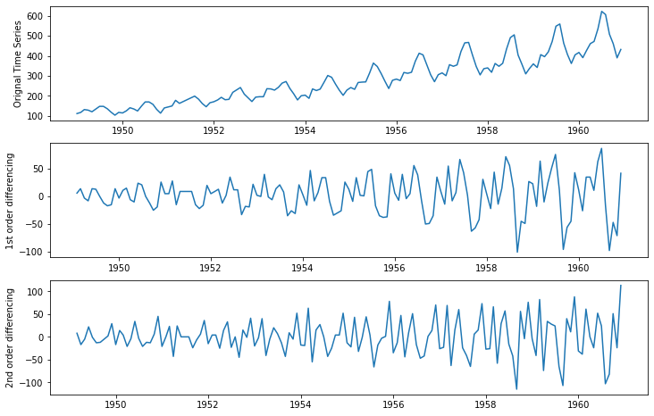
In the diagram shown above, we can observe that the time series is showing an increasing trend over time, differencing technique is used to eliminate this trend by subtracting the value of the previous observation from the current observation.

At the first difference level, it still has a linear trend but we have successfully removed the higher-order trend observed in the original time series. After the 2nd difference level, the series obtained is mostly a horizontal line. There is no overall visible trend in this series and thus we can say the series obtained is a stationary series.

This has created a new time series of the differences between consecutive observations, which can be analyzed and modeled as a stationary time series.

Transformation

So far we have discussed a differencing method that helps in making mean constant. In the same way, the other method to introduce stationarity is making the variance constant by applying transformations. Transformation involves applying mathematical functions to the time series data to stabilize the mean and variance.

There can be many transformation methods used to make a non-stationary series stationary but here, we will be discussing the Box-Cox transformation. The mathematical formula for the Box-cox transformation is:

$$y(\lambda) = {y^\lambda - 1 \over \lambda}, if \lambda \ne 0$$

And,

$$y(\lambda) = {log\lambda }, if \lambda = 0$$

where y is the original time series and y(λ) is the transformed series. The procedure for the Box-Cox transformation is to find the optimal value of λ between -5 and 5 (as this range covers a wide variety of power transformations that can be applied to the data) that minimizes the variance of the transformed data.

NOTE: The optimal value of lambda for a particular dataset depends on the distributional characteristics of the data and the specific modeling objectives. Therefore, the lambda value should be chosen based on statistical methods such as maximum likelihood estimation or through trial and error experimentation.

Let us look at a Python example to apply the Box-Cox transformation to make variance constant.

from scipy.stats import boxcox
data_boxcox = pd.Series(boxcox(data['Passengers'], lmbda=0), index = data.index)

plt.figure(figsize=(12,4))
plt.plot(data_boxcox, label='After Box Cox tranformation')
plt.legend(loc='best')
plt.title('After Box Cox transform')
plt.show()

Other transformations include square root transformation, power transformation, and logarithmic transformation. The choice of transformation method depends on the characteristics of the time series data and the specific modeling objectives.

Autocorrelation

The second assumption of the AR-based model is autocorrelation.

Correlation refers to a statistical measure that quantifies the degree to which two or more variables are related or associated with each other. We check how strongly the dependent variables and independent variables are correlated to each other. In the same way, autocorrelation is about capturing the movement of past observations (which can be thought of as independent variables) and impacts future observations (which can be thought of as dependent variables).

In simple terms, autocorrelation is capturing the relationship between observations \(y_t\) at time t and \(y_{t-k}\) at time k period before t. It helps us to know how a variable is influenced by its own lagged values.

We will look at two autocorrelation measures Autocorrelation function (ACF) and Partial autocorrelation function (PACF). Let us start discussing the same.

Autocorrelation function (ACF)

ACF stands for the Autocorrelation function, which is a statistical function used to measure the degree of correlation between a time series and its lagged values. The ACF is a plot of the correlation coefficient (r) against the lag (k) at different lags.

The ACF measures how closely related a time series observation is to its lagged values. For example, if the ACF at lag k is high, then it means that the value at time t is highly correlated with the value at time t-k, indicating that there is a pattern in the data that repeats every k time step.

Let us understand with the help of an example how the autocorrelation function helps in determining the correlation between an observation with its lagged values.

Once we have calculated the lags, we next plot the ACF plot for the observation value and the lag values.

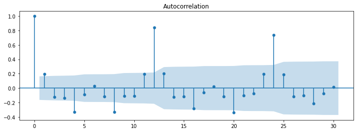
Here in the diagram shown above, autocorrelation is calculated for the multiple lags. We can also see that the current observation is significantly correlated with lag 12 and lag 24.

One interesting thing to notice is that ACF measures the correlation between a time series and its lagged values, including all intermediate lags. It shows the correlation between the current value of the time series and its past values at all possible lags.

Partial autocorrelation function (PACF)

PACF is different from ACF where it measures the correlation between a time series and its lagged values, after removing the effect of the intermediate lags. It shows the correlation between the current value of the time series and its past values at specific lags, without taking into account the effect of the other lags.

In summary, ACF measures the correlation at all lags while PACF measures the correlation at specific lags after removing the effect of the intermediate lags.

Deep diving into AR-based models

After having an understanding of the assumptions of the AR-based models. Let's talk about actual stuff and dive straight into the different types of AR models that we can use to solve for time series data. In this post, we will be covering six different Auto-Regressive models as follows:

1. Auto-Regressive (AR)
2. Moving Average (MA)
3. Auto-Regressive Moving Average (ARMA)
4. Auto-Regressive Integrated Moving Average (ARIMA)
5. Seasonal Auto-Regressive Integrated Moving Average(SARIMA).
6. Seasonal Auto-Regressive Integrated Moving Average with Exogenous variable (SARIMAX)

Let's discuss them in detail.

Simple Auto-Regressive model (AR)

The Simple Auto-Regressive model predicts the future observation as the linear regression of one or more past observations. In simpler terms, the simple autoregressive model forecasts the dependent variable (future observation) when one or more independent variables are known (past observations). This model has a parameter ‘p’ called lag order. Lag order is the maximum number of lags used to build the ‘p’ number of past data points to predict future data points. 

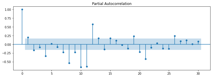
The plot partial autocorrelation function is used to find the p-value and the autocorrelation model equation is built. From the partial autocorrelation function plot, we select p as the highest lag where partial autocorrelation is significantly high.

Once the lags are identified which have high autocorrelation, the next step is to build a regression equation. Consider an example PACF plot shown below:

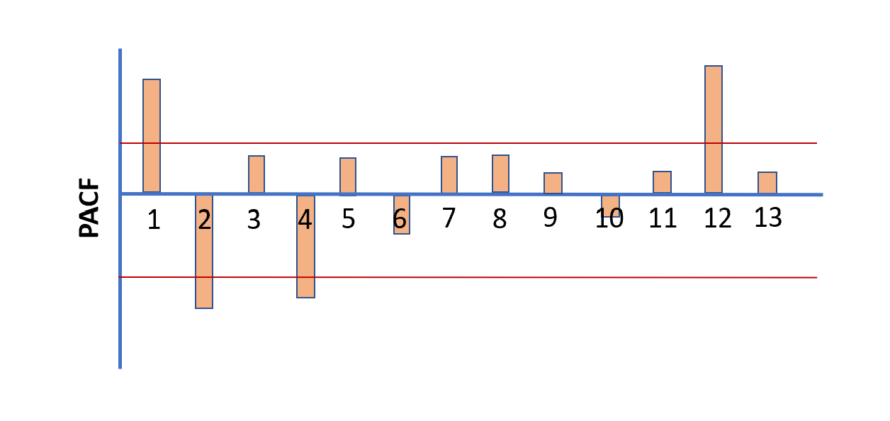
Here, the lag value of 1, 2, 4, and 12 has a significant level of confidence. i.e., a significant level of influence on future observation (refer to the red line). Hence, the value of 'p' will be set to 12 since that is the highest lag where partial autocorrelation is significantly high.

Therefore, the autoregression model equation will be:

$$\hat y = \beta_0 +  \beta_1y_{t-1} + \beta_1y_{t-2} + \beta_1y_{t-4} + \beta_1y_{t-12}$$

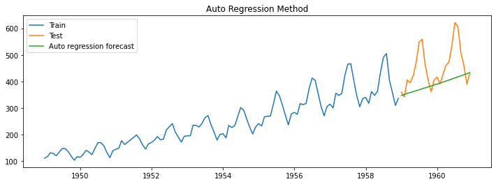
Let us consider a sample code to build an AR model with the lag order as 1.

from statsmodels.tsa.arima_model import ARIMA
model = ARIMA(train_data_boxcox_diff, order=(1, 0, 0)) 
model_fit = model.fit()

The below image represents the output from the model.

Moving Average model (MA)

In contrast to an AR model, which uses past values of the time series to predict future values, an MA model uses past error terms to predict future values. The idea behind the MA model is that the current value of the time series depends on the weighted sum of the past error terms.

The equation of the MA model is:

$$\hat y = \mu + \phi_1 \epsilon_{t-1}$$

where \(\epsilon_{t-1}\) represents the error from the previous prediction and \(\phi_1\) is coefficient multiplied to error term.

Let us take an example, where we want to predict the number of passengers that will be traveling business class. Let's say on day 1 we started with the prediction of 30 as from historical data we know that the average number of passengers flying business class is 30, but then the actual business class passengers were 27, therefore having an error rate of 3.

Now for the next day, we will predict using the MA model to be mean along with a percentage of error of the previous day's prediction. i.e., 30 + 0.5(-3) = 28.5 assuming the coefficient to be 0.5.

NOTE: The predictions will always move around 30 and this is the reason why this model is called the Moving average model. Here, the primary goal is to predict the plus and minus variation that can be observed over a period of time. 

This model has a parameter ‘q’ called window size over which a linear combination of errors is calculated. In the example discussed above, we have taken a 'q' value of 1 as we have calculated only the last forecast error to determine the next forecast.

Now the question arises, how do we determine the q variable? To determine the value of parameter ‘q’, we plot the Autocorrelation function (ACF).

We start by plotting the Autocorrelation function (ACF) and select q as the highest lag beyond which autocorrelation dies down.

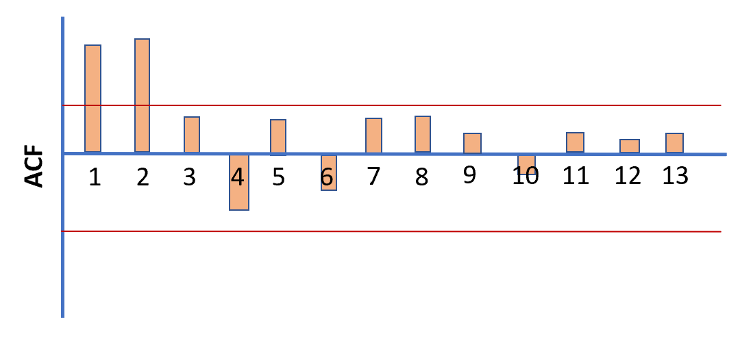
For the above-shown ACF plot, we see that 2 is the highest lag beyond which autocorrelation dies down. Therefore, the equation of the MA model will be:

$$\hat y = \mu + \phi_1 \epsilon_{t-1} + \phi_2 \epsilon_{t-2}$$

Let us consider a sample code to build an AR model with a window size of 1.

model = ARIMA(train_data_boxcox_diff, order=(0, 0, 1)) 
model_fit = model.fit()
print(model_fit.params)

Auto-Regressive Moving Average (ARMA)

The ARMA model assumes that the current value of the time series is a linear combination of its past values and past error terms. This model is a combination of AR and MA models. Therefore we use both PACF and ACF to find the value for p and q respectively.

ARMA model equation with values of p and q as 1 will be represented as:

$$\hat y = \beta_0 + \beta_1y_{t-1} + \phi_1 \epsilon_{t-1}$$

where \(\beta_1\) and \(\phi_1\) are the coefficients, \(y_{t-1}\) is the lagged observation and \(\epsilon_{t-1}\) is the forecast error of last time period.

Let us consider a sample code to build an ARMA model with a lag order of 1 and a window size of 1.

model = ARIMA(train_data_boxcox_diff, order=(1, 0, 1))
model_fit = model.fit()
print(model_fit.params)

Auto-Regressive Integrated Moving Average (ARIMA)

The AR-based models discussed so far are built using a stationary series. Suppose now we have a series with a trend in it and we want to build a model on this dataset directly. How we will do this?

ARIMA (Auto-Regressive Integrated Moving Average) model is a variation of the ARMA model that takes into account non-stationarity in the data by introducing a differencing term that helps to remove trends from the data. The three terms in the ARIMA acronym represent the following:

1. AutoRegressive (AR)
2. Integrated (I)
3. Moving Average (MA)

We have already discussed AR and MA models. Integrated (I) refers to the differencing of the time series to make it stationary. The order of the differencing term specifies how many times the series is differenced.

NOTE: It is important to note that ARIMA model still cannot handle if time series is non stationary because fo variance in the data. It can only handle time series data which is non stationary and has trend but variance is constant.

The steps involved to build the ARIMA model are as follows:

• The original time series is differenced to make it stationary. Basically to remove the variance from the data.
   
• Differenced series is modeled as a linear regression of
  • One or more past observations which are the same as AR models
  • Past forecast error which is the same as MA models
     
• Along with the 'p' and 'q' parameters that we have discussed there is also a third parameter 'd' which signifies the degree of differencing to make the series stationary.
   
• The choice of 'd' value should be to make the series stationary. We can run hit and trail and further verify if this differenced series is stationary or not by using the stationarity tests: ADF or KPSS test.
   
• The last step in the ARIMA model is to recover the original time series forecast.

Let us next write an equation for the ARIMA model with p,d, and q values as 1.

$$Z_t = \phi_1Z_{t-1} + \theta_1\epsilon_{t-1} + \epsilon_t$$

Doesn't this equation look similar to the ARMA equation with the only difference that here we have Z in this equation and y in the ARMA equation? Yes, that's correct and this is because \(Z_t\) here represents the differenced series. Therefore,

$$Z_t = y_{t+1} - y_t$$

\(Z_t\) here represents the first-order differenced series.

Python code to build the ARIMA model:

model = ARIMA(train_data_boxcox, order=(1, 1, 1))
model_fit = model.fit()

Fundamentally speaking ARIMA model is no different than the ARMA model. For the ARMA model, we have to apply both the boxcox transformation and differencing to convert the data into stationary time-series data. But for the ARIMA model, we are just applying boxcox before building the model and letting the model take care of the differencing i.e. the trend component itself.

Therefore output should fundamentally be the same for both ARMA and ARIMA models.

Seasonal Auto-Regressive Integrated Moving Average (SARIMA)

SARIMA is the model which captures the seasonality which no other models discussed so far captured. SARIMA brings all the features of an ARIMA model with an extra feature - seasonality. Let's next identify the building blocks of the SARIMA model.

• As one would expect it brings all the nonseasonal elements of the ARIMA models.
• In addition, it has seasonal elements that are added to the model.

Therefore to build a SARIMA model we first have to consider non-seasonal components like ARIMA. We also have to perform seasonal differencing on time series to make the seasonal component of the time series stationary. And thereafter we have to model future seasonality as the linear regression of past observations of seasonality and past forecast errors of seasonality.

Therefore along with non-seasonal 'p', 'd', and 'q' parameters which we in ARIMA models, there are further seasonal parameters 'P', 'D', 'Q', and 'm' which are required to build the SARIMA model. 'P', 'D', and 'Q' are seasonal lag order, difference order, and window size; and 'm' is the number of time steps for a single seasonal period.

We figure out the value of the non-seasonal parameters exactly in the same way we did earlier in the ARIMA model, but to find the seasonal parameters ('P', 'D', 'Q') we use grid search and the 'm' parameter is something that we should know from data or business.

Let us next write an equation for the SARIMA model represented as \(SARIMA(1,0,0)(0,1,1)_4\) where p is 1, d and q are 0, P is 0 and D and Q are 1, and m is 4.

$$Z_t = \beta_1Z_{t-1} + \phi\epsilon_{t-4} + \epsilon_t$$

Here \(\beta_1Z_{t-1}\) represent the no-seasonal p value, \(\phi\epsilon_{t-4} \) represent the seasonal q value. Wherever we see t - 4, we can think of it as a seasonal term since in our case seasonality is 4.

Further, since we don't have a nonseasonal differencing term but we only have a seasonal differencing term. Therefore \(Z_t\) is represented as:

$$Z_t = y_{t} - y_{t-4} $$

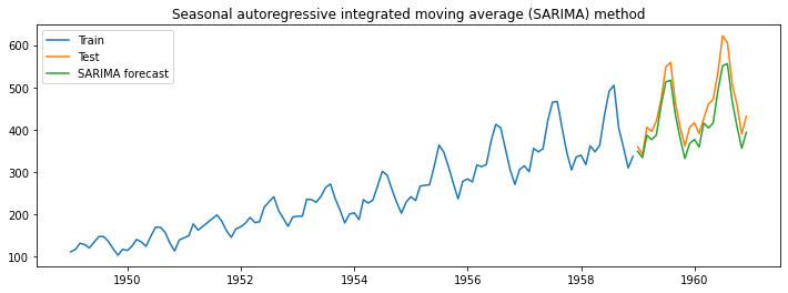
Python code to build the SARIMA model:

from statsmodels.tsa.statespace.sarimax import SARIMAX

model = SARIMAX(train_data_boxcox, order=(1, 1, 1), seasonal_order=(1, 1, 1, 12)) 
model_fit = model.fit()

The below image represents the output from the model.

Seasonal Auto-Regressive Integrated Moving Average with Exogenous variable (SARIMAX)

SARIMAX is an autoregressive model which models an external variable along with the non-seasonal and seasonal components. Or in other words SARIMA with exogenous variables. It has three components:

• Non-seasonal elements (same as that of the ARIMA model)
• Seasonal elements (same as that of the SARIMA model)
• Exogenous variable (Additional feature that gets added to the model)

Let us next write an equation for the SARIMA model represented as \(SARIMAX(1,0,0)(0,1,1)_4\).

$$Z_t = \beta Z_{t-1} + \phi\epsilon_{t-4} + \alpha x_t$$

$$Z_t = y_{t} - y_{t-4} $$

The equation is the same as that of the ARIMA model with the only difference being that the alpha terms are added here.

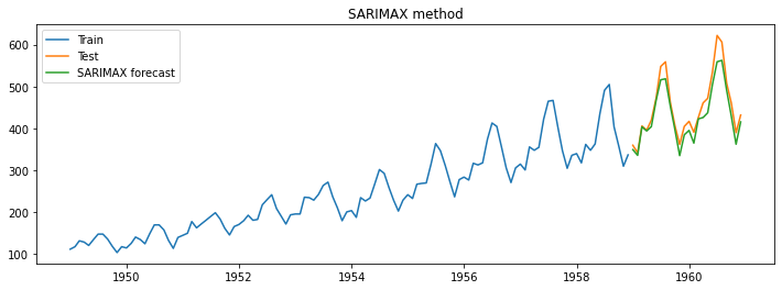
Python code to build the SARIMAX model:

model = SARIMAX(train_data_boxcox, order=(1, 1, 1), seasonal_order=(1, 1, 1, 12), exog=promo_train) 
model_fit = model.fit()

The below image represents the output from the model.

Summary

In part 1 and part 2 of the article "Guide to build accurate Time Series Forecasting Models", we have discussed various time series models that can be used for different types of data. The time series smoothing-based models that we have discussed are:

1. Naive method
2. Simple average method (SA)
3. Simple moving average method (SMA)
4. The simple exponential smoothing technique (SES)
5. Holt’s exponential smoothing technique (HES)
6. Holt-Winters’ exponential smoothing technique (HWES)

We have further discussed the autoregressive model-based models such as:

1. Auto-Regressive method (AR)
2. Moving Average method (MA)
3. Autoregressive moving average method (ARMA)
4. Autoregressive integrated moving average method (ARIMA)
5. Seasonal autoregressive integrated moving average method (SARIMA)
6. Seasonal Auto-Regressive Integrated Moving Average with Exogenous variable (SARIMAX)

NOTE: There are further vector based time series models such as Vector Autoregression (VAR), Vector Autoregression Moving-Average (VARMA), and Vector Autoregression Moving-Average with Exogenous Regressors (VARMAX) which are not discussed in this post.

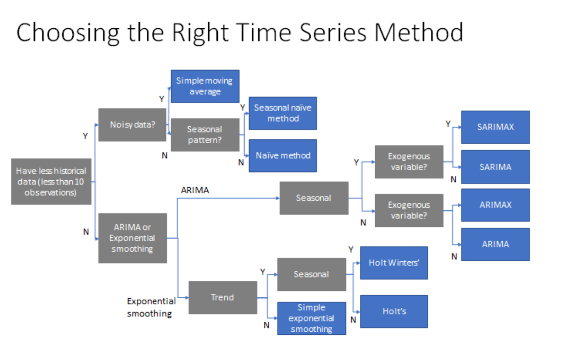
One common question, that we may have as we are closing the post is, It's great to have so many options available to build time series models, but how to decide which model to choose for my use case?

This post has got you covered. The below diagram specifies certain thumb of rules that one can follow to choose the right algorithm based on the data available. 

I hope you have enjoyed this two parts post on building an accurate time series model. I have also created a Jupyter Notebook for reference if you get blocked or want to run the code shared in the blog locally.